2 Mixed-strategy Nash equilibrium
2.1 Why randomize?
In the previous chapter, matching pennies and the household-chores game had no pure-strategy Nash equilibrium. At every pure profile, someone could improve their payoff by changing their choice. This does not mean that these games have no equilibrium once players can randomize. It means that a fixed choice of a pure strategy may be too restrictive.
In matching pennies, a predictable choice can be exploited. A probability distribution over heads and tails allows a player to specify how they will randomize without making the realized choice predictable. The relevant question becomes: can the players choose distributions such that neither benefits from changing their own distribution?
This chapter develops the definitions and mathematical conditions needed to answer that question. Throughout, the normal-form game \(\left(N,(S_i)_{i\in N},(u_i)_{i\in N}\right)\) is finite, that is, every \(S_i\) is a finite strategy set. We retain \(\mathbf S=\prod_{i\in N}S_i\) and the notation \(\mathbf s_{-i}\) for the opponents’ pure strategies.
2.2 Mixed strategies and expected utility
2.2.1 Probability distributions over pure strategies
A player first selects a distribution and then draws a pure strategy according to it. The draws of different players are independent. Thus the probability of the pure profile \(\mathbf s\) is
\[ \prod_{i\in N}p_i(s_i). \]
Randomization does not require repeated play, although repeated independent draws make its frequencies easier to observe.
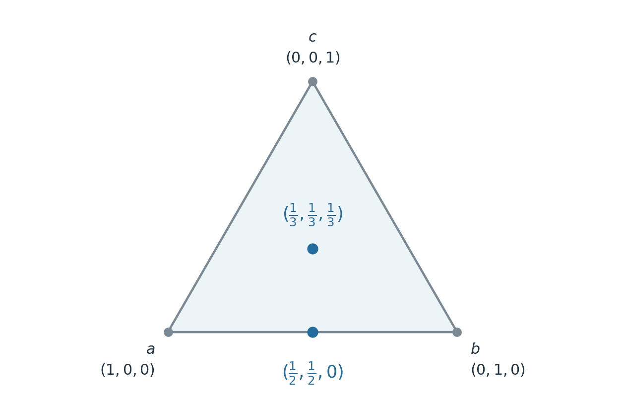
We identify a pure strategy \(s_i\) with the distribution assigning probability \(1\) to \(s_i\) and \(0\) otherwise. Consequently, pure strategies are special cases of mixed strategies. For example, if \(S_i=\{H,T\}\), a mixed strategy can be written as \((p,1-p)\), with \(0\le p\le1\). The endpoints are pure strategies. For \(S_i=\{a,b,c\}\), the set \(\Delta_i\) is a triangle, namely the probability simplex in Figure 2.1. Its vertices are pure strategies. Every edge contains distributions using at most two pure strategies. More generally, for \(|S_i|=m\), the simplex has dimension \(m-1\).
2.2.2 Expected utility
A rational player seeks to maximize expected utility.
We use the following notation: lowercase \(u_i\) evaluates a pure profile and uppercase \(U_i\) evaluates a mixed profile. In particular, against opponents’ distributions \(\mathbf p_{-i}\), the expected utility of a pure strategy \(s_i\) is
\[ U_i(s_i,\mathbf p_{-i}) =\sum_{\mathbf s_{-i}\in\mathbf S_{-i}} u_i(s_i,\mathbf s_{-i})\prod_{j\ne i}p_j(s_j). \]
Regrouping (2.1) by player \(i\)’s choice gives the identity used throughout this chapter:
\[ U_i(p_i,\mathbf p_{-i}) =\sum_{s_i\in S_i}p_i(s_i)U_i(s_i,\mathbf p_{-i}). \tag{2.2}\]
For fixed opponents’ strategies, a player’s expected utility is a weighted average of the utilities of their pure strategies. In particular, it is linear in that player’s own probabilities.
2.3 Nash equilibrium and best responses
The comparison holds the opponents’ distributions fixed. A deviation may change any of player \(i\)’s probabilities, including replacing randomization by a pure strategy. Equilibrium rules out a strictly profitable deviation.
2.3.1 The best-response correspondence
For fixed \(\mathbf p_{-i}\), define
\[ \operatorname{BR}_i(\mathbf p_{-i}) =\underset{p_i\in\Delta_i}{\operatorname{argmax}} U_i(p_i,\mathbf p_{-i}). \]
The set-valued map \(\operatorname{BR}_i\) is the best-response correspondence. Its value \(\operatorname{BR}_i(\mathbf p_{-i})\) is the set of mixed strategies of player \(i\) that are best responses to \(\mathbf p_{-i}\). Directly from the definitions,
\[ \mathbf p^*\text{ is a Nash equilibrium} \quad\Longleftrightarrow\quad p_i^*\in\operatorname{BR}_i(\mathbf p_{-i}^*) \text{ for every }i\in N. \]
2.3.2 Why pure strategies suffice to test Nash equilibrium
Although there are infinitely many mixed strategies, there are only finitely many pure strategies to test if a given mixed strategy profile is an equilibrium.
Proof. Necessity follows because pure strategies are mixed strategies. Conversely, suppose all the displayed inequalities hold. For any mixed strategy \(p_i\), identity (2.2) gives
\[ \begin{aligned} U_i(p_i,\mathbf p_{-i}^*) &=\sum_{s_i\in S_i}p_i(s_i)U_i(s_i,\mathbf p_{-i}^*)\\ &\le\sum_{s_i\in S_i}p_i(s_i)U_i(\mathbf p^*)=U_i(\mathbf p^*)\sum_{s_i\in S_i}p_i(s_i) =U_i(\mathbf p^*). \end{aligned} \] \(\square\)
2.4 Existence of equilibrium
The proof uses a fixed-point theorem. We use the existence result here without reproducing that proof. Several qualifications matter. A mixed strategy includes a pure strategy, so the theorem does not assert that some player must randomize. It provides only an existence guarantee. The methods for finding an equilibrium belong to the later topic on computing Nash equilibrium.
2.5 Supports and indifference
For example, let \(S_i=\{a,b,c\}\) and \(p_i(a)=p_i(b)=p_i(c)=\frac 13\), then \(p_i\) is completely mixed. Another mixed strategy \(q_i(a)=q_i(b)=\frac 12\) has support \(\operatorname{spt}(q_i)=\{a,b\}\). A pure strategy has a one-element support.
2.5.1 The indifference principle
Proof. Suppose \(s_i,t_i\in\operatorname{spt}(p_i^*)\) and \(U_i(s_i,\mathbf p_{-i}^*)>U_i(t_i,\mathbf p_{-i}^*)\). Transfer all probability assigned to \(t_i\) to \(s_i\), leaving the other probabilities unchanged. Specifically, define:
\[ p_i(a)= \begin{cases} 0,&a=t_i,\\ p_i^*(s_i)+p_i^*(t_i),&a=s_i,\\ p_i^*(a),&a\notin\{s_i,t_i\}. \end{cases} \]
This is a mixed strategy. Its improvement in expected utility is
\[ U_i(p_i,\mathbf p_{-i}^*)-U_i(\mathbf p^*) =p_i^*(t_i)\bigl[U_i(s_i,\mathbf p_{-i}^*) -U_i(t_i,\mathbf p_{-i}^*)\bigr]>0, \]
contradicting equilibrium. Therefore the utilities on the support are equal. Their weighted average is \(U_i(\mathbf p^*)\), so their common value must be that expected utility. \(\square\)
The reason for mixing is therefore not that a weighted average improves on the best pure reply. A player mixes among equally good replies, and the chosen probabilities in turn affect the opponents’ incentives.
In conclusion, indifference among strategies in the support is necessary but not sufficient for equilibrium: we must also check that no strategy outside the support gives a higher payoff.
2.5.2 The support characterization
Indifference among used pure strategies is necessary for an equilibrium. The question remains if an unused strategy outside the support might still be better. To state the necessary and sufficient condition for equilibrium, distinguish pure from mixed best responses:
\[ B_i(\mathbf p_{-i}) =\underset{s_i\in S_i}{\operatorname{argmax}} U_i(s_i,\mathbf p_{-i}). \]
The set \(B_i(\mathbf p_{-i})\) consists of pure strategies, whereas \(\operatorname{BR}_i(\mathbf p_{-i})\) consists of probability distributions. Since \(S_i\) is finite, \(B_i(\mathbf p_{-i})\neq \emptyset\).
Proof. Let \(\mathbf p^*\) be an equilibrium. For any pure strategy \(s_i\in \operatorname{spt}(p_i^*)\), the indifference principle says that \[ U_i(s_i,\mathbf p_{-i}^*) = U_i(\mathbf p^*). \] For any pure strategy \(s_i \in S_i\setminus \operatorname{spt}(p_i^*)\), the pure deviation condition is \[ U_i(s_i,\mathbf p_{-i}^*) \le U_i(\mathbf p^*) \] Therefore, \[ U_i(\mathbf p^*) = \max_{s_i\in S_i} U_i(s_i,\mathbf p_{-i}^*), \] which proves inclusion (2.3).
Conversely, let (2.3) hold for a profile \(\mathbf p^*\). Then \[ \begin{aligned} U_i(\mathbf p^*) & = \sum_{s_i \in \operatorname{spt}(p_i^*)} p_i^*(s_i)U_i(s_i,\mathbf p_{-i}^*)=\sum_{s_i \in \operatorname{spt}(p_i^*)} p_i^*(s_i)\max_{t_i\in S_i}U_i(t_i,\mathbf p_{-i}^*) \\ & = \max_{t_i\in S_i}U_i(t_i,\mathbf p_{-i}^*) \cdot \sum_{s_i \in \operatorname{spt}(p_i^*)} p_i^*(s_i)=\max_{t_i\in S_i}U_i(t_i,\mathbf p_{-i}^*), \end{aligned} \] where (2.3) was used in the second equality. The derived identity \[ U_i(\mathbf p^*) = \max_{t_i\in S_i}U_i(t_i,\mathbf p_{-i}^*) \] means that \(\mathbf p^*\) is a Nash equilibrium. \(\square\)
Equivalently, condition (2.3) says that for every player \(i\):
- every strategy in the support gives expected utility \(U_i(\mathbf p^*)\);
- every strategy outside the support gives expected utility at most \(U_i(\mathbf p^*)\).
The inclusion (2.3) need not be equality: an unused pure strategy outside the support is allowed to tie with those in the support. If the profile is completely mixed, there are no unused strategies, so indifference for every player is sufficient.
2.6 Two-player \((2\times2)\) examples
This case is elementary. Let \(p\) and \(q\) denote the players’ probabilities of choosing their first strategies. The indifference principle gives two linear equations: solve for \(q\) by making the row player indifferent, and for \(p\) by making the column player indifferent. If \(0<p,q<1\), they define a completely mixed strategy profile and hence an equilibrium.
2.7 Good Samaritan: Who will provide aid?
This example is adapted from the Good Samaritan Game in Chapter 2 of Binmore’s Game Theory: A Very Short Introduction (Binmore 2007, 25–26). There are \(n\ge2\) bystanders who hear a cry for aid. Each independently chooses whether to provide aid (\(a\)) or leave the task to someone else (\(\bar a\)), without observing the others’ choices. Everyone values someone receiving help at \(10\) utility units. Providing aid costs \(1\) utility unit, so a helper receives \(9\) regardless of how many others also help. A non-helper receives \(10\) if someone else helps and \(0\) if nobody helps.
Thus \(S_i=\{a,\bar a\}\) and
\[ u_i(\mathbf s)= \begin{cases} 9,&s_i=a,\\ 10,&s_i=\bar a\text{ and some }j\ne i\text{ chooses }a,\\ 0,&\mathbf s=(\bar a,\ldots,\bar a). \end{cases} \]
For \(n=2\), the game is
\[ \begin{array}{c|cc} & a & \bar a \\ \hline a & 9, 9 & 9, 10 \\ \bar a & 10, 9 & 0, 0 \end{array} \]
2.7.1 Pure equilibria
There are exactly \(n\) pure equilibria, each with exactly one helper:
- If nobody helps, any bystander can increase their utility from \(0\) to \(9\) by helping.
- If at least two bystanders help, any helper can stop helping and increase their utility from \(9\) to \(10\).
- If exactly one helps, that helper would lose \(9\) by stopping, while every other bystander would lose \(1\) by also helping.
Pure equilibria therefore exist, but they assign different roles to identical players. The model by itself does not select the helper.
2.7.2 A symmetric mixed equilibrium
We now look for a particular equilibrium in which everyone uses the same distribution. This is a restriction on the equilibrium we seek, not a consequence that every equilibrium must satisfy. Let \(q\) be each bystander’s probability of not helping and \(\mathbf p\) be the corresponding strategy profile. Then
\[ U_i(a,\mathbf p_{-i})=9, \qquad U_i(\bar a,\mathbf p_{-i})=10\bigl(1-q^{n-1}\bigr). \]
For both pure strategies to be used with positive probability, indifference requires
\[ 9=10\bigl(1-q^{n-1}\bigr), \qquad q=(0.1)^{1/(n-1)}. \]
Since \(0<q<1\), this gives a completely mixed profile. This shows that the profile is a Nash equilibrium with
\[ U_i(\mathbf p^*)=9\qquad\text{for every }i\in N. \]
2.7.3 The chance that nobody helps
There are \(n-1\) other bystanders in an individual’s indifference condition, but there are \(n\) bystanders who must all abstain for aid to fail. Consequently, at the symmetric equilibrium,
\[ \Pr(\text{nobody helps})=q^n=(0.1)^{n/(n-1)}. \]
| Bystanders \(n\) | Each player’s probability of helping \(1-q\) | Probability nobody helps \(q^n\) |
|---|---|---|
| \(2\) | \(0.900\) | \(0.010\) |
| \(3\) | \(0.684\) | \(0.032\) |
| \(5\) | \(0.438\) | \(0.056\) |
| \(10\) | \(0.226\) | \(0.077\) |
As \(n\to\infty\),
\[ q\longrightarrow1,\qquad 1-q\longrightarrow0,\qquad q^n\longrightarrow0.1. \]
Each individual becomes less likely to help as the group grows. The chance of no aid increases toward \(10\%\) in this family of symmetric equilibria, even though there are more potential helpers. This is a consequence of the specified incentives and independent equilibrium randomization, rather than an empirical claim about actual emergencies.