Two Thirds of the Average
The target in this game depends on the numbers chosen by the players. To choose well, a player must think about what the others will choose and how they will reason. The game provides a concrete connection between the normal-form model, best responses, dominance, and Nash equilibrium introduced in the textbook.
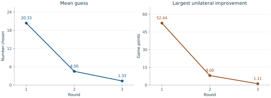
This chapter analyses the distance-payoff version played in class, then examines the recorded choices of six players over three rounds. The mean guess moved from approximately \(20.33\) to \(4.50\) to \(1.33\). This is movement toward the zero equilibrium, although none of the three observed profiles was an equilibrium and the number of exact zero choices actually decreased.
Rules and classroom procedure
Each player privately chooses a real number in \([0,100]\). All guesses are submitted before any current-round submissions are revealed. The instructor computes the arithmetic mean of all valid guesses and takes two thirds of that mean as the target. Every player earns 100 minus their absolute distance from the target. The objective is to maximize one’s own game points.
The classroom procedure used three rounds with \(6\) players. In each round, players made their individual choices. After seeing the guesses, mean, target, and scores, they made another individual choice. This repeated until the third round, when the total results were revealed.
The analysis below concerns the one-round game. In the three-round activity, a full strategy would specify choices following possible histories of feedback and discussion. Repeating the game supplies experience, while it does not by itself guarantee that play will approach an equilibrium.
Relation to the beauty-contest game
The classic experiment in Nagel (1995) awards a fixed prize to the player closest to the target, divided equally in a tie. That is a different payoff rule. Continuous payoffs based on absolute distance are studied by Güth et al. (2002). Our model is a specialization of their general family. The best responses here are derived for the distance payoff and must not be transferred to a winner-only prize rule.
Normal-form model
For \(n\ge2\), use the textbook notation
\[ \left(N,(S_i)_{i\in N},(u_i)_{i\in N}\right), \qquad N=\{1,\ldots,n\},\qquad S_i=[0,100]. \]
The strategy profile space is \(\mathbf S=[0,100]^n\). For a profile \(\mathbf s=(s_1,\ldots,s_n)\), write
\[ \bar s=\frac1n\sum_{i\in N}s_i, \qquad T(\mathbf s)=\frac23\bar s. \]
The utility functions are
\[ u_i(\mathbf s)=100-|s_i-T(\mathbf s)|, \qquad i\in N. \tag{1}\]
This is an infinite, symmetric, non-cooperative, and general-sum game in normal form. Its rules and payoffs are announced to every player. The model assumes that each player maximizes their own points.
Best response
Fix \(i\in N\) and an opponents’ profile \(\mathbf s_{-i}\). Let
\[ A_{-i}=\sum_{j\ne i}s_j. \]
Expanding the term in the absolute value in Equation 1 gives
\[ \begin{aligned} s_i-T(\mathbf s) &=s_i-\frac{2}{3n}(s_i+A_{-i})\\ &=\frac{3n-2}{3n}s_i-\frac{2}{3n}A_{-i}\\ &=\frac{3n-2}{3n} \left(s_i-\frac{2A_{-i}}{3n-2}\right). \end{aligned} \]
Define
\[ r_i(\mathbf s_{-i})=\frac{2A_{-i}}{3n-2}. \]
The payoff can therefore be written as
\[ u_i(\mathbf s) =100-\frac{3n-2}{3n}|s_i-r_i(\mathbf s_{-i})|. \]
The coefficient is positive, so the unique maximum occurs at \(s_i=r_i(\mathbf s_{-i})\), provided this number is feasible. It is feasible because
\[ 0\le r_i(\mathbf s_{-i}) \le100\frac{2(n-1)}{3n-2}<100. \]
Following the set-valued definition in Equation 1.2, the best-response is unique, so that
\[ \operatorname{BR}_i(\mathbf s_{-i}) =r_i(\mathbf s_{-i})=\frac{2}{3n-2}\sum_{j\ne i}s_j. \tag{2}\]
Every such response earns 100 points. Writing \(\bar s_{-i}=A_{-i}/(n-1)\) and
\[ q=\frac{2(n-1)}{3n-2}, \]
we also have \(\operatorname{BR}_i(\mathbf s_{-i})=q\bar s_{-i}\), where \(q < 2/3\), although \(q\) approaches \(2/3\) as \(n\) grows.
Nash equilibrium
Proof. Clearly, when all opponents choose zero, the choice zero gives 100 points to player \(i\). Any deviation to \(0< t_i\leq 100\) gives
\[ u_i(t_i,\mathbf0_{-i}) =100-\left(1-\frac{2}{3n}\right)t_i<100. \]
Thus no unilateral deviation is profitable. Conversely, at a Nash equilibrium, each player must choose their unique best response in Equation 2:
\[ s_i^*=\frac23\bar s^*\qquad\text{for every }i\in N. \]
Averaging these equalities yields
\[ \bar s^*=\frac23\bar s^*, \qquad\text{so}\qquad \bar s^*=0. \]
Consequently every \(s_i^*\) equals zero. \(\square\)
Note that the zero is not a weakly dominant strategy. Against opponents all choosing 50, the unique best response is the positive number \(50q\). Choosing zero instead gives
\[ u_i(0,50,\ldots,50)=100-\frac{100(n-1)}{3n}<100. \]
There is no weakly dominant strategy at all. Indeed, only zero is optimal against all-zero opponents, whereas zero is not optimal against all-50 opponents.
Why two thirds rather than the average?
Replace the multiplier \(2/3\) by \(p\). For \(0<p<1\), on the same strategy sets \([0,100]\) the analogous calculation gives \[ \operatorname{BR}_i(\mathbf s_{-i}) =\frac{p}{n-p}\sum_{j\ne i}s_j, \qquad q_p=\frac{p(n-1)}{n-p}<1. \]
The unique equilibrium remains all zero. Thus two thirds is a convenient conventional choice and its particular value is not essential for these conclusions.
If \(p=1\), players try to match the average itself. The best-response set is then the singleton containing the opponents’ average. Therefore, every unanimous profile \((c,\ldots,c)\), \(c\in[0,100]\), is a pure Nash equilibrium. These are all the pure equilibria, because equilibrium requires \(s_i=\bar s\) for every \(i\).
Agreement on a positive number creates an incentive to move lower for \(p<1\). For example, a conjectured opponents’ mean of 50 leads to roughly 33, then 22, then 15 under successive large-population reasoning with \(p=2/3\); with \(p=1\) the corresponding anchor stays at 50.
Changing the strategy interval
Now suppose every player has the same compact strategy interval \(S_i=[a,b]\), where \(a<b\), and the target is still \(p\bar s\) with \(0<p<1\). The payoff remains \(100-|s_i-p\bar s|\), but this score can be negative. Changing the additive constant 100 would not change any best response or equilibrium.
A constrained best response
The unconstrained ideal strategy is still
\[ r_i(\mathbf s_{-i})=\frac{p}{n-p}\sum_{j\ne i}s_j =q_p\bar s_{-i}, \]
but it may now lie outside the feasible interval. Define the projection
\[ \Pi_{[a,b]}(x)=\min\{b,\max\{a,x\}\}. \]
Maximizing utility now means choosing the feasible strategy nearest to \(r_i\):
\[ \operatorname{BR}_i(\mathbf s_{-i}) =\Pi_{[a,b]} \left(\frac{p}{n-p}\sum_{j\ne i}s_j\right). \tag{3}\]
The equilibrium is the feasible point nearest zero
Proof. We will introduce this simplified notation first. Let \(F_i(\mathbf s)\) be the right-hand side of Equation 3. At the unanimous profile \(\mathbf s=(c,\ldots,c)\), we get \(F_i(\mathbf s)=\Pi_{[a,b]}(q_pc)=c\), so this profile is an equilibrium.
Projection onto an interval cannot increase distances of the arguments. Therefore, for any two profiles \(\mathbf s,\mathbf t\),
\[ \begin{aligned} |F_i(\mathbf s)-F_i(\mathbf t)| &\le\frac{p}{n-p}\sum_{j\ne i}|s_j-t_j|\\ &\le q_p\|\mathbf s-\mathbf t\|_\infty, \end{aligned} \]
where \(\|\mathbf s-\mathbf t\|_\infty=\max_i|s_i-t_i|\). If both profiles were equilibria, they would be fixed points of \(F\), yielding
\[ \|\mathbf s-\mathbf t\|_\infty \le q_p\|\mathbf s-\mathbf t\|_\infty. \]
Since \(q_p<1\), this forces \(\mathbf s=\mathbf t\). \(\square\)
The six-player classroom record
The following analysis contains six valid submissions in each of three rounds.
Choices
| Player | Round 1 guess | Round 2 guess | Round 3 guess |
|---|---|---|---|
| P01 | 28 | 11 | 1 |
| P02 | 1 | 1 | 2 |
| P03 | 0 | 3 | 1 |
| P04 | 66 | 0 | 1 |
| P05 | 0 | 3 | 2 |
| P06 | 27 | 9 | 1 |
Observed scores
| Player | Round 1 score | Round 2 score | Round 3 score |
|---|---|---|---|
| P01 | 85.5556 | 92 | 99.8889 |
| P02 | 87.4444 | 98 | 98.8889 |
| P03 | 86.4444 | 100 | 99.8889 |
| P04 | 47.5556 | 97 | 99.8889 |
| P05 | 86.4444 | 100 | 98.8889 |
| P06 | 86.5556 | 94 | 99.8889 |
We summarize the results across the three rounds using selected statistics.
| Statistic | Round 1 | Round 2 | Round 3 |
|---|---|---|---|
| Sum | \(122\) | \(27\) | \(8\) |
| Mean | \(61/3\approx20.3333\) | \(9/2=4.5\) | \(4/3\approx1.3333\) |
| Target | \(122/9\approx13.5556\) | \(3\) | \(8/9\approx0.8889\) |
| Smallest and largest guess | \(0,66\) | \(0,11\) | \(1,2\) |
| Number of zero guesses | \(2\) | \(1\) | \(0\) |
| Mean score | \(80\) | \(581/6\approx96.8333\) | \(896/9\approx99.5556\) |
Measuring the remaining incentive to deviate
Define player \(i\)’s unilateral improvement at the observed profile as
\[ \begin{aligned} R_i(\mathbf s) &=\max_{t_i\in S_i} \bigl[u_i(t_i,\mathbf s_{-i})-u_i(\mathbf s)\bigr]\\ &=100-u_i(\mathbf s). \end{aligned} \]
The second equality holds here because a feasible best response always earns 100 points. The maximum improvement
\[ \varepsilon(\mathbf s)=\max_i R_i(\mathbf s) \]
is zero exactly at a Nash equilibrium. More generally, a profile is an \(\varepsilon\)-Nash equilibrium if no player can improve their utility by more than \(\varepsilon\). For each recorded round we get
\[ \varepsilon(\mathbf s^{(1)})=472/9\approx52.4444, \qquad \varepsilon(\mathbf s^{(2)})=8, \qquad \varepsilon(\mathbf s^{(3)})=10/9\approx1.1111. \]
Thus the final profile is a \(10/9\)-Nash equilibrium in the stated score units, but not an exact Nash equilibrium. This quantifies the remaining incentive to deviate.
For completeness, the exact ex post best responses in all rounds are:
| Player | Round 1 best response | Round 2 best response | Round 3 best response |
|---|---|---|---|
| P01 | \(47/4\) | \(2\) | \(7/8\) |
| P02 | \(121/8\) | \(13/4\) | \(3/4\) |
| P03 | \(61/4\) | \(3\) | \(7/8\) |
| P04 | \(7\) | \(27/8\) | \(7/8\) |
| P05 | \(61/4\) | \(3\) | \(3/4\) |
| P06 | \(95/8\) | \(9/4\) | \(7/8\) |
These are retrospective comparisons with the realized opponents’ choices fixed. Players did not observe those choices when submitting, so an ex post improvement does not by itself establish an unreasonable prior belief or an irrational decision.
What the record supports
The mean guess and the maximum guess both decrease, so the observed profiles move closer to \((0,\ldots,0)\) in both average and maximum absolute distance. The spread also narrows, from the observed range \([0,66]\) to \([1,2]\). Meanwhile, the mean and maximum unilateral improvements decrease sharply. These are complementary signs of movement toward equilibrium over the three observed rounds.
The number of exact equilibrium actions, however, falls from two to one to zero. Counting zero guesses would miss the aggregate movement. Individual paths are heterogeneous: P01 and P06 decrease throughout, P02 finishes above their initial choice, and P03 and P05 first leave zero. These patterns show why the analysis should examine whole profiles and incentives, rather than assigning a reasoning level to a single number.